Robotics

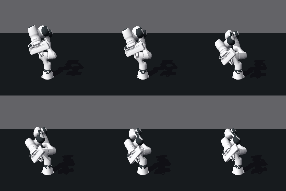
xwm.envs wraps a Franka Emika FR3 in Newton (NVIDIA Warp), observed either as pixels or as a 20-D proprioceptive state vector. A dense reach task supplies the reward the value-based families need.

pip install "xwm[newton]"

The robot asset is fetched on first use, so the first construction is slower than the rest.

One episode under a smoothed action sequence. The arm is what the reward is computed from; the goal is a point in space it has to reach.

The environment

env = xwm.envs.FrankaEnv(xwm.envs.FrankaConfig(image_size=64))

env.reset(seed=0)
env.step(action)                 # (7,) joint deltas, scaled by config.action_scale

env.observe()                    # (3, 64, 64) pixels -- what a vision model sees
env.state_observation()          # (20,) joints, velocities, tool, goal delta
env.reward(action)               # dense, roughly [-1, 0], minus an action penalty
env.goal_distance()              # metres, ground truth -- for evaluation only

env.action_dim is 7, env.state_dim is 20. The reward is \(-\tanh(\text{distance})\) rather than \(-\text{distance}\): a bounded reward keeps the value function inside the categorical head's bin range without per-task tuning, and its gradient does not vanish far from the goal the way a squared distance's does.

State first, pixels later

TD-MPC2 and MuZero on the 20-D state converge in minutes rather than hours, which makes them testable. Get the pipeline working there, then swap in an image encoder. The family code does not change.

Configuration

FrankaConfig is a dataclass; the fields worth knowing:

field	default	what it changes
image_size	64	resolution of observe()
action_scale	0.25	how far one action moves each joint
goal	(0.3, 0.15, 0.55)	the reach target, in metres
pose_noise	0.35	spread of the initial pose across resets
action_penalty	0.01	coefficient on \(\lVert a \rVert\) in the reward
enable_shadows / enable_textures	False	renderer fidelity, for figures
solver	"auto"	mujoco_warp where a CUDA GPU is available, Featherstone otherwise
fps, substeps	30, 16	simulation timestep and stability

Data for a JEPA

franka_sequences returns exactly what xwm.data.sprite_sequences does, so it drops straight into any family:

data = xwm.envs.franka_sequences(env, 2048, 8, seed=0)   # 2048 episodes of 8 frames
data["video"].shape      # (2048, 8, 3, 64, 64)
data["action"].shape     # (2048, 7, 7)   -- action[i, t] joins frames t and t + 1
data["joint_q"].shape    # (2048, 8, 7)   ground truth, for probes only
data["tool"].shape       # (2048, 8, 3)   hand position, for probes only

Diverged rollouts, meaning a NaN out of the solver, are discarded and resampled, so the dataset never contains a corrupt sequence.

One sequence: eight frames and the seven actions between them. Rendered at 768 px per frame, shown here at about a twelfth of that, so open it full size to see the arm articulate. The encoder is given the same frames at config.image_size.

Actions are smoothed (smoothness=0.7) rather than i.i.d. uniform, because independent per-step noise produces jitter, and a jittering arm visits a much smaller region of the state space than a drifting one does. Pass progress_every=100 if you want progress printed, since a couple of thousand episodes takes a while on CPU.

The two-stage recipe

Learn a representation from passive observation, freeze it, learn action-conditioned dynamics in its latent space:

# 1. Representation, from observation alone.
jepa = xwm.families.jepa.lejepa(size="small", img_size=64, patch_size=8, reg_weight=5.0)
state, _ = xwm.training.Trainer(jepa, xwm.training.adamw(1e-3)).fit(frames, steps=4000)

# 2. Dynamics, in that frozen latent space.
world = xwm.families.jepa.action_world_model(
    action_dim=env.action_dim, encoder=state.model.encoder, freeze_encoder=True,
    img_size=64, patch_size=8,
)
state, _ = xwm.training.Trainer(world, xwm.training.adamw(1e-4)).fit(clips, steps=6000)

Then plan toward a goal image:

planner = xwm.planning.CEM(horizon=5, action_dim=7, n_samples=512, n_elites=64)
cost = xwm.planning.goal_cost(world.encode(goal_image), kind="l2", action_penalty=0.05)

plan = planner.plan(key, world.dynamics_fn(), world.encode(env.observe()), cost)
env.step(plan.actions[0])

Measured over the held-out episodes (findings):

policy	mean (m)	% of gap closed	mean |a|
no-op	0.246	0.0	n/a
random	0.345	−39.8	n/a
planner (a_pen=0)	0.220	+10.7	0.213
planner (a_pen=0.05)	0.193	+21.6	0.090

The action penalty is not a cosmetic regulariser: it doubled the gap closed and more than halved the action magnitude. A planner with nothing to lose will thrash.

Quote the range, not the headline

Three runs at this identical preset closed +28%, +12% and +22%, so the effect is roughly 21% with a spread as large as itself, and the honest claim is 10–30%. What replicates across all three is the ordering and the action penalty's sign. See the variance finding.

Reward-driven instead

With a reward available, skip the two stages:

TD-MPC2MuZero

agent = xwm.families.tdmpc2.tdmpc2(
    action_dim=env.action_dim, observation="state", state_dim=env.state_dim,
)
planner, cost = xwm.families.tdmpc2.planner(agent)

table = xwm.envs.discrete_action_table(env.action_dim)   # (15, 7)
agent = xwm.families.muzero.muzero(
    n_actions=len(table), observation="state", state_dim=env.state_dim,
)

discrete_action_table is the bridge from a 7-DoF arm to a discrete-action algorithm: ± on each joint, plus a no-op.

Determinism, and why it matters for figures

The physics is deterministic given a seed and an action sequence:

result = env.rollout(actions, seed=0)
result["video"]      # (T + 1, 3, H, W) -- the initial frame precedes the first action
result["joint_q"]    # (T + 1, 7)  ground truth, for probes
result["tool"]       # (T + 1, 3)  hand position, for probes

So a path-traced figure is produced by replaying an episode rather than by storing its pixels, and the render is therefore of the same episode the numbers came from.

For a stochastic policy this needs one more step, and it is the reason the Franka examples share examples/_common.py::figure_episode. TD-MPC2's MPPI and MuZero's MCTS do not return the same action twice, so re-running the policy for a second renderer would produce a different episode that merely looks similar. The helper drives the episode once, records the actions it took, and replays those recorded actions for every other renderer:

figure_episode(
    env, out,
    policy=lambda e: act(e.state_observation()),   # MPPI or MCTS, stochastic
    steps=EPISODE_LEN, seed=10_000,
    label="TD-MPC2 planning on the Franka reach task",
)

One episode then underlies the GIF, the frame strip and the USD stage, and the policy is evaluated exactly as many times as the episode has steps. See Rendering.

Health check

Newton can diverge, given a pathological action sequence:

if not env.is_finite():
    env.reset(seed=...)

Worth checking in a collection loop. A NaN in the buffer poisons every batch that touches it.