Avoiding collapse¶

Predicting a representation from a representation has a trivial solution: emit a constant. Both sides of the loss then agree perfectly and the model has learned nothing. The collapse= argument on JEPA selects the countermeasure; each recipe fixes one.

option	used by	mechanism	teacher?
`"ema"`	I-JEPA, V-JEPA	targets from a slowly-moving copy, gradients cut	yes
`"sigreg"`	LeJEPA	a distributional penalty forbids the constant solution	no
`"vicreg"`	VICReg	variance + covariance penalties	no
`"none"`	n/a	control, for watching collapse happen	no

The recipes cover the two strategies worth training with:

model = xwm.families.jepa.ijepa(img_size=64)                    # collapse="ema"
model = xwm.families.jepa.lejepa(img_size=64, reg_weight=5.0)   # collapse="sigreg"

For "vicreg" or "none", whether for a comparison or a deliberate look at the failure, build the JEPA yourself. A recipe is a convenient way to get the three parts:

base = xwm.families.jepa.ijepa(img_size=64, patch_size=8)

model = xwm.JEPA(
    base.encoder, base.predictor, base.mask_sampler, input_key="image",
    collapse="vicreg", reg_weight=1.0,
)

SIGReg¶

SIGReg replaces EMA teachers, stop-gradients, centering and sharpening with one statement: the embedding distribution should be an isotropic Gaussian.

It is enforced by a sketch. For \(z \sim \mathcal{N}(0, I_D)\) and any unit vector \(v\), the projection \(\langle z, v \rangle\) is exactly \(\mathcal{N}(0, 1)\), regardless of \(D\). So draw random directions, project the batch onto each, and penalise deviation from a standard normal:

xwm.objectives.sigreg(z, key, n_proj=256, statistic="epps_pulley")

Isotropy and unit scale both fall out of that one test, the cost is linear in batch size, and there is one coefficient instead of a schedule. Two statistics are available: "epps_pulley" (a characteristic-function test, the default) and "cramer_von_mises".

Why this is more than a convenience

An EMA teacher is a moving target, and its momentum is a schedule you have to tune. SIGReg has no teacher, so the target is the data: the same objective at step 1 and step 100 000. That is what makes reg_weight the only knob.

What it costs to skip¶

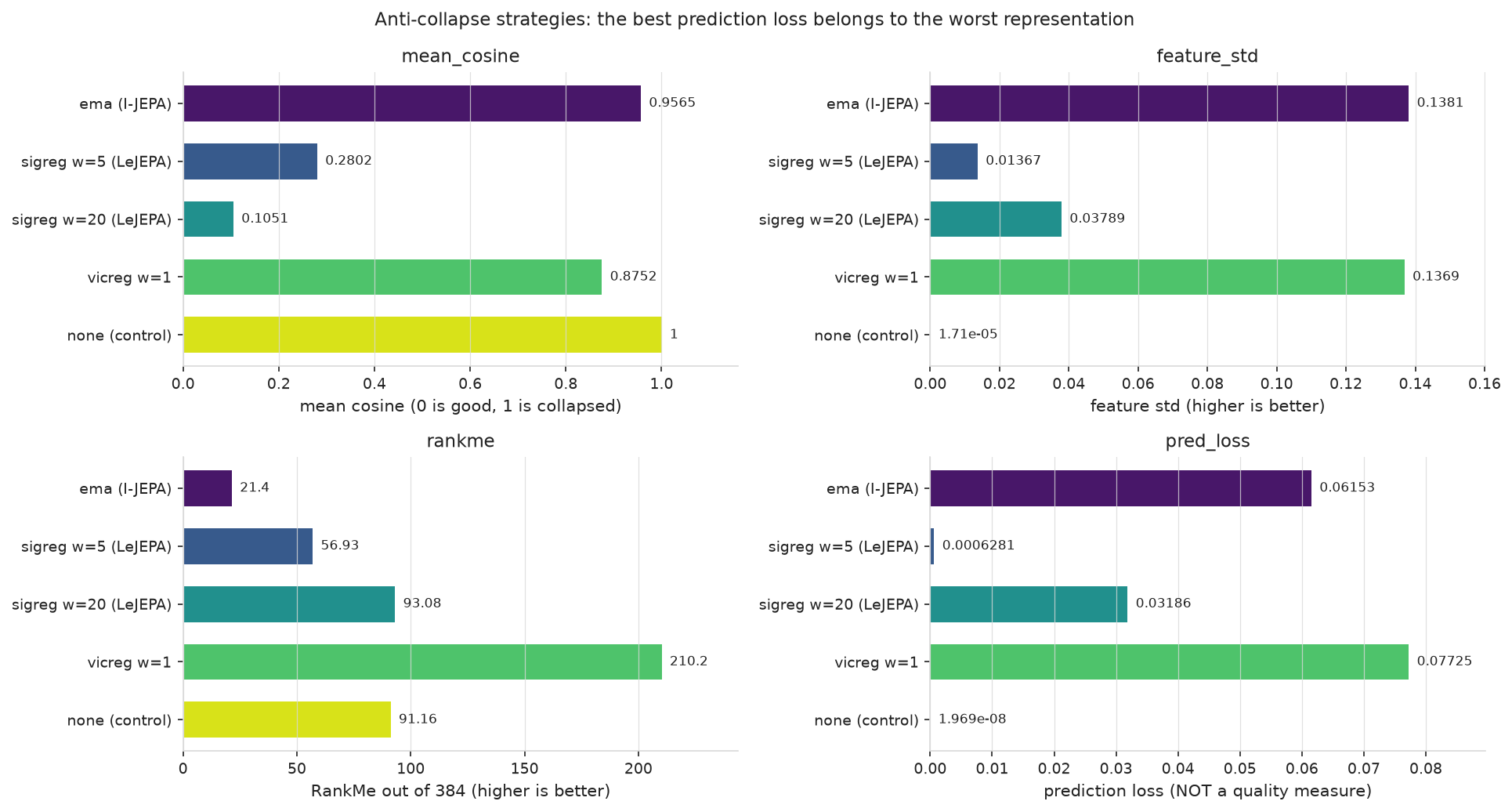
Measured on 2048 sprite images, 4000 steps, 384-dim embeddings (full table):

strategy	pred_loss	feature_std	mean_cosine	rankme (of 384)	probe R²
ema (I-JEPA)	0.0615	0.138	0.957	21.4	0.188
sigreg w=5 (LeJEPA)	0.00063	0.014	0.280	56.9	0.941
sigreg w=20 (LeJEPA)	0.0319	0.038	0.105	93.1	0.960
vicreg w=1	0.0772	0.137	0.875	210.2	0.329
none (control)	2e-08	1.7e-05	1.000	91.2	0.982

Read the control row first. Its prediction loss is the best on the page by seven orders of magnitude, its mean_cosine is 1.000, and it has learned nothing at all, because every embedding is the same vector. Lower prediction loss does not mean a better representation.

The EMA row is the honest cost of the teacher mechanism at this scale: on a task this easy, mean_cosine = 0.957 means it has largely collapsed too, and its probe R² is the worst of the four real strategies. SIGReg at w=20 is what a healthy run looks like: the highest effective rank of the non-degenerate rows, the lowest mean cosine, and the best probe.

Diagnostics across anti-collapse strategies — Four strategies, four diagnostics. The strategy with the lowest loss is the one that learned nothing.

VICReg¶

VICReg attacks collapse from the other end: a variance term pushes each feature's standard deviation toward 1, and a covariance term pushes off-diagonal feature correlations toward 0.

loss, metrics = xwm.objectives.vicreg(z_a, z_b, sim_coeff=25.0, var_coeff=25.0, cov_coeff=1.0)

It works, and the table above shows the highest raw rankme of any row, but the rank is spread thin: mean_cosine stays at 0.875 and the probe only reaches 0.329. Three coefficients also mean three things to tune, which is the practical argument for SIGReg.

Watching it happen¶

collapse="none" exists for exactly one purpose: to see the failure, so you recognise it in a run where you did not ask for it.

model = xwm.JEPA(base.encoder, base.predictor, base.mask_sampler, collapse="none")
# then watch feature_std -> 0 and mean_cosine -> 1

examples/03_collapse_strategies.py runs all four side by side. What to measure is in Diagnostics.