Planning

A planner needs two things: a way to imagine, and a way to score what it imagined. xwm keeps both deliberately narrow.

step = model.dynamics_fn()                                  # (z, a) -> z'
cost = xwm.planning.goal_cost(model.encode(goal), kind="l2") # (z, a, t) -> scalar

planner = xwm.planning.CEM(horizon=8, action_dim=7, n_samples=512, n_elites=64)
plan = planner.plan(key, step, model.encode(observation), cost)

plan is a Plan: plan.actions is (horizon, action_dim), plan.mean is the refined distribution to warm-start the next call with.

That is the whole contract. A planner never sees the model, the encoder, the observation or a reward function, only a closure and a cost. That is why one implementation of each planner serves all three families.

The planners

planner	actions	notes
CEM	continuous	samples whole sequences, keeps the elites, refits
MPPI	continuous	softmax-weights every sample by cost instead of hard-selecting
GradientPlanner	continuous	differentiates the rollout; happy to exploit model error
MCTS	discrete	grows a PUCT tree; what MuZero uses

CEM and MPPI are what JEPA and TD-MPC2 use. The gradient planner is included because it is instructive: it finds the model's optimum, which on an imperfect model is often an action sequence the real system cannot follow, which is to say adversarial examples against your own dynamics.

One device call

Everything in xwm.planning is jittable. Candidates are vmaped and refinement is a lax.fori_loop, so a plan is a single device call rather than a Python loop over samples:

import equinox as eqx

@eqx.filter_jit
def solve(key, z0, z_goal):
    return planner.plan(key, step, z0, xwm.planning.goal_cost(z_goal, kind="l2"))

The cost is built inside the jitted function, because a cost is a closure. Pass it in as an argument and JAX has nothing to trace.

This is why the horizon and the sample count are constructor arguments rather than call arguments: they are static shapes.

Costs

A cost is (z, a, t) -> scalar. It sees the latent, the action that produced it and the timestep, so discounting and action penalties are expressible without special-casing.

cost	scores by
goal_cost	latent distance to a goal embedding
reward_cost	a learned reward head
return_cost	discounted reward plus a terminal value bootstrap
sum_costs	a weighted sum of any of the above

cost = xwm.planning.goal_cost(z_goal, kind="l2", action_penalty=0.05, discount=0.99)

action_penalty is worth a moment: it costs a little goal progress and buys much smaller actions. On the Franka reach task, a_pen=0.05 closed 21.6% of the gap with mean \(|a|\) of 0.090, against 10.7% and 0.213 for the unpenalised planner (findings): better and less than half as violent, because a planner with no penalty will happily thrash. Large opposing actions cancel in the true dynamics, but the model scores them as progress. This is the one Franka result that came out the same way in every run.

Seeing past the horizon

return_cost is the term that lets a horizon-3 planner act as though it saw further:

cost = xwm.planning.return_cost(
    lambda z, a: reward.value(z, a),                    # learned reward head
    lambda z: critic.pessimistic(z, policy.act(z)),     # terminal value bootstrap
    horizon=3, discount=0.99,
)

TD-MPC2 wires this for you: xwm.families.tdmpc2.planner(model) returns the (planner, cost) pair already pointed at the model's own heads.

Without the value bootstrap, a 3-step planner optimises 3 steps of reward and is blind to everything after. With it, the terminal latent is scored by a learned value, which is the whole point of the value-based families.

Closing the loop

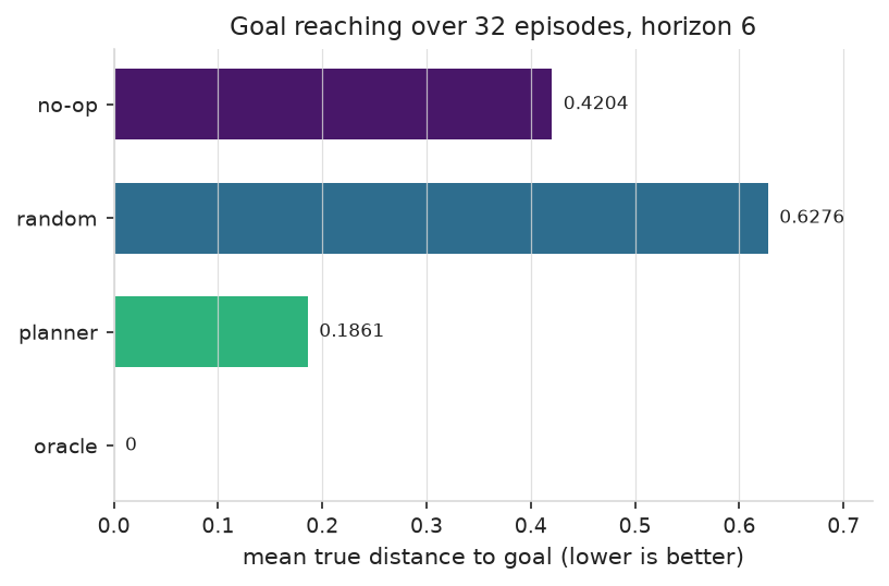
A plan computed once is open-loop. run_mpc replans at every step and warm-starts from the previous solution:

observations, actions, plans = xwm.planning.run_mpc(
    key, planner, model.dynamics_fn(), cost,
    encode=model.encode, step_env=env.step, observation=obs0, n_steps=20,
)

shift_plan is the warm start (roll the previous mean forward one step), and control_step is one plan-act-observe cycle if you want to drive the loop yourself.

The planner against no-op, random and an oracle, over 32 episodes of the synthetic world. It optimises a latent cost and never sees a true position.

Discrete actions

MCTS takes the same dynamics closure, plus the reward, value and policy heads that guide the search:

search = xwm.planning.MCTS(n_actions=15, n_simulations=50, c_puct=1.25)
recurrent, predict = model.search_fns()

result = search.search(key, model.represent(observation), recurrent, predict)

result.action        # the visit-count argmax
result.policy        # the visit distribution -- MuZero's policy target
result.value         # the root value estimate

model.search_fns() returns the (recurrent, predict) pair the tree needs: \((s, a) \rightarrow (s', r)\) and \(s \rightarrow (\pi, v)\). If your actions are continuous but you want a tree, discrete_action_table gives you a fixed set of primitives to search over, which is how MuZero drives a 7-DoF arm.