Diagnostics

The loss is not the metric. A collapsing encoder drives its prediction loss down, because it is predicting its own degenerate output, and a constant is very easy to predict. In the collapse comparison the run with the best loss by seven orders of magnitude had learned nothing at all.

So measure the representation:

xwm.metrics.collapse_report(z)
# {'rankme': ..., 'rank_ratio': ..., 'feature_std': ..., 'mean_cosine': ...}

What each one catches

metric	collapsed when	measures
feature_std	→ 0	per-dimension spread across inputs
mean_cosine_similarity	→ 1	how alike two random embeddings are
rankme	→ 1	effective rank of the spectrum
effective_rank_ratio	→ 0	the same, as a fraction of embed_dim

All four are reported because each misses a case the others catch:

• rankme is computed after centring, so a large constant offset is invisible to it: a representation can be rank-rich around a mean it never departs from.
• feature_std is per-dimension, so it does not see a representation that varies a lot along one direction and not at all along the rest.
• mean_cosine is scale-invariant, so it does not see a representation whose spread is collapsing uniformly.

Read them together. feature_std → 0 and mean_cosine → 1 is the unambiguous signature.

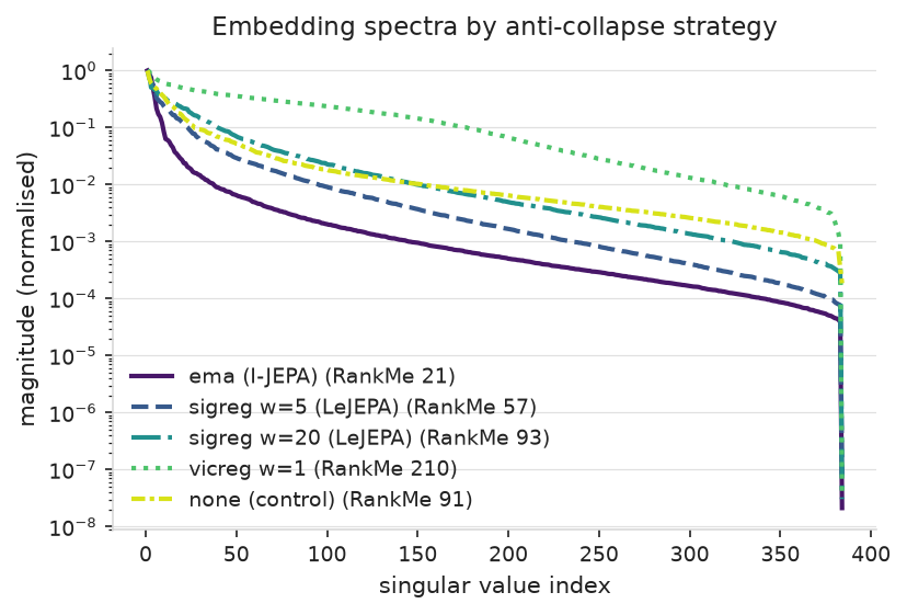
Singular-value spectra of the same encoder trained five ways. A healthy representation decays slowly; a collapsed one falls off a cliff.

singular_values gives you the spectrum itself, and xwm.plots.plot_spectra draws it.

A probe is not a collapse detector

This is the trap worth internalising. ridge_probe standardises features before fitting, so it divides by a near-zero standard deviation and amplifies a nearly-dead signal back to full scale.

Measured on the sprite world, the fully collapsed control run scored R² = 0.982, the highest probe score in the comparison (findings).

scores = xwm.metrics.ridge_probe(z_train, y_train, z_test, y_test)
scores["r2"]      # tells you what is linearly decodable, not whether z is healthy

Use a probe for what it is good at: is the information I care about linearly available? Then ask collapse_report whether the representation is alive.

And beware an easy target

On the synthetic sprite world the agent's position is nearly a linear function of the red channel, so the probe saturates before training even begins: R² = 0.999 on a randomly initialised encoder. examples/01_image_ijepa.py prints the before-and-after side by side precisely to show that.

k-NN, for when linear is too generous

xwm.metrics.knn_probe(z_train, y_train, z_test, y_test, k=5)

A k-NN probe asks whether the neighbourhood structure carries the label, which no amount of feature standardisation can fake. It is slower and it needs a sensible metric, but it is much harder to fool.

In a training loop

The Trainer logs whatever a model's loss returns as metrics. Most families include an embedding-spread term (embed_std, latent_std) for exactly this reason, so collapse is visible while it happens rather than after:

state, history = trainer.fit(
    batches, steps=1000,
    callbacks=[xwm.training.print_metrics(every=50, keys=["loss", "embed_std"])],
)

Then check the representation properly at the end, on held-out data:

embed = jax.jit(jax.vmap(state.model.embed))
z = xwm.core.batched_apply(embed, held_out["image"], batch_size=64)

for name, value in xwm.metrics.collapse_report(z).items():
    print(f"{name:<12} {float(value):.4f}")

Diagnostics for a dynamics model

Representation health is only half of it. A world model also has to be right about the future, and the honest test is a free rollout against a no-op baseline: predict \(h\) steps from a single latent, consuming its own predictions:

z_pred = model.imagine(z0, actions)          # (T, ...) -- no ground truth after z0

horizon	model L1	no-op L1	ratio
1	0.0570	0.0588	0.97
3	0.0723	0.0998	0.72
7	0.0911	0.1235	0.74

A ratio below 1 means the model beats assuming nothing changes, which is a surprisingly strong baseline at short horizons, and the reason a raw L1 number is uninterpretable on its own. Full tables in Findings.