JEPA

Predict masked latents without collapsing. A JEPA learns a representation by predicting its own embeddings at positions it was not shown. No reward, no reconstruction, which means it trains on passive observation, and there is a great deal more of that than there is of labelled interaction.

model = xwm.families.jepa.lejepa(size="small", img_size=224, patch_size=16)

The recipes

recipe	grid	collapse	follows
ijepa	2-D patches	EMA teacher	I-JEPA
lejepa	2-D patches	SIGReg	LeJEPA
vjepa	3-D tubelets	EMA teacher	V-JEPA
video_lejepa	3-D tubelets	SIGReg	LeJEPA on clips

Each assembles an encoder, a JEPAPredictor and a mask sampler into a JEPA, and fixes the anti-collapse strategy. size= picks a ViT preset (tiny, small, base or large), and encoder_kwargs / predictor_kwargs override any of it:

model = xwm.families.jepa.ijepa(
    size="tiny", img_size=64, patch_size=8,
    n_targets=4, target_scale=0.15,
    encoder_kwargs={"depth": 4, "embed_dim": 128, "num_heads": 4},
    predictor_kwargs={"depth": 3, "pred_dim": 64, "num_heads": 4},
)

How the loss works

1. prepare_batch samples a mask on the host, outside jit: one context, several target blocks.
2. The context encoder runs on the visible tokens only. This is where the speedup over reconstruction comes from.
3. The predictor maps context tokens plus target positions to predicted target embeddings.
4. Targets come from the teacher: an EMA copy of the encoder with gradients cut (collapse="ema"), or the encoder itself plus a distributional penalty (collapse="sigreg").

loss, metrics = model.loss(batch, key=key)
metrics        # {'loss': ..., 'pred_loss': ..., 'reg': ..., 'embed_std': ...}

embed_std is the one to watch while it trains. See Diagnostics.

Avoiding collapse

This is the whole difficulty of the family, and it has its own page: Collapse. The short version: ijepa uses an EMA teacher, lejepa uses SIGReg and needs no teacher at all, and on a small dataset the EMA teacher collapses too.

From representation to robot

A JEPA has no actions. The V-JEPA 2-AC recipe adds them in a second stage: freeze the encoder, learn action-conditioned dynamics in its latent space.

model = xwm.families.jepa.action_world_model(
    action_dim=7, encoder=pretrained_encoder, freeze_encoder=True,
)

trainer = xwm.training.Trainer(model, xwm.training.adamw(1e-4))
trainer.n_trainable == model.dynamics.n_params   # the encoder gets no optimizer state

Freezing is not only a compute saving

With the encoder fixed, the prediction targets are fixed functions of the observations. So the dynamics model has nothing to gain from degrading the representation. The shortcut where the encoder quietly makes itself easier to predict is closed off by construction.

Two training terms

ActionWorldModel.loss mixes them:

term	one step from	penalises
teacher forcing	ground-truth latents	single-step error, a dense signal
rollout	its own predictions, whole horizon	compounding error

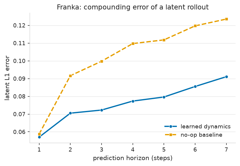
Only the rollout term sees compounding error, and only teacher forcing gives a dense per-step gradient, so both are needed. Measured on the Franka arm, a free rollout beats a no-op baseline out to seven steps (findings):

Held-out latent L1 of a free rollout, against "assume nothing changes". The ratio, not the absolute error, is the interpretable quantity.

Then plan

planner = xwm.planning.CEM(horizon=8, action_dim=7, n_samples=512, n_elites=64)
cost = xwm.planning.goal_cost(model.encode(goal_image), kind="l2")

plan = planner.plan(key, model.dynamics_fn(), model.encode(observation), cost)

The goal is an image. Encode it, and the distance to it in latent space is the cost. No reward function, no state estimation, no coordinates anywhere. See Planning.

Video

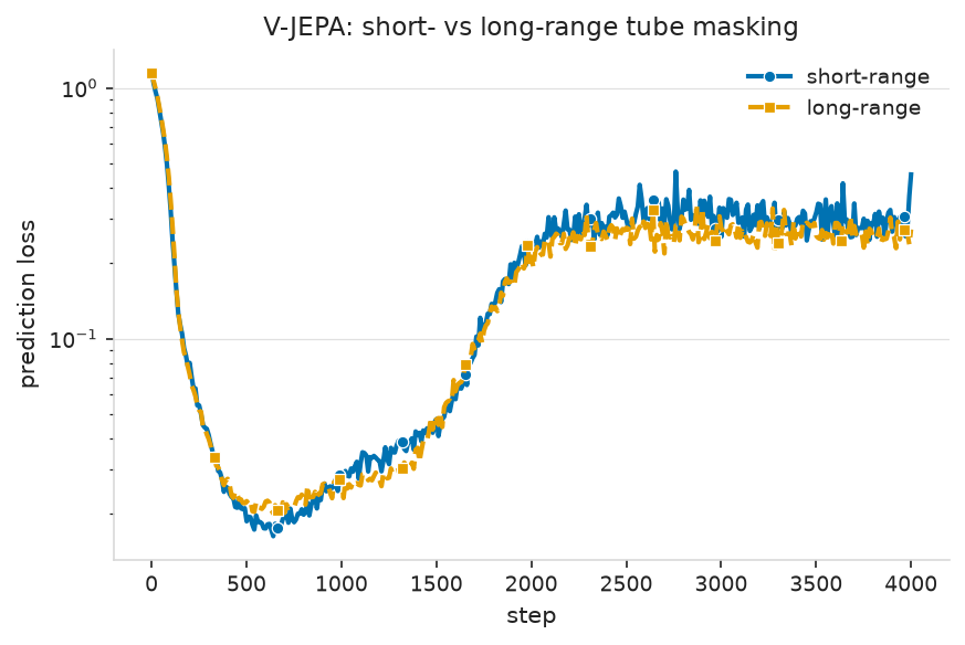
vjepa and video_lejepa work over 3-D tubelets with TubeMask3d, whose whole purpose is to ensure no visible frame contains the answer:

model = xwm.families.jepa.vjepa(
    size="small", img_size=128, patch_size=16, num_frames=8, tubelet_size=2,
    n_targets=2, spatial_scale=0.15,
)

Short-range (many small tubes) against long-range (few large ones). The long-range preset reaches both the lower loss and the higher effective rank.

Examples

example	shows
01_image_ijepa.py	I-JEPA pretraining, a probe, collapse diagnostics
02_video_vjepa.py	tube masking, short- vs long-range
03_collapse_strategies.py	ema vs sigreg vs vicreg vs none
04_action_world_model.py	frozen encoder + latent dynamics, compounding error
05_planning.py	the full JEPA pipeline, measured against baselines

See Examples.