Concepts

A world model answers "what happens if I do this?". An action-conditioned one answers it in a latent space of its own choosing, which is what makes it usable for robotics: you can search over imagined action sequences without rendering a single pixel.

Three pieces and no decoder

Three learned pieces, one of which is optional. The encoder runs once per observation; the dynamics model runs once per imagined step; the heads read scalars and distributions off a latent. Nothing maps Z back to O.

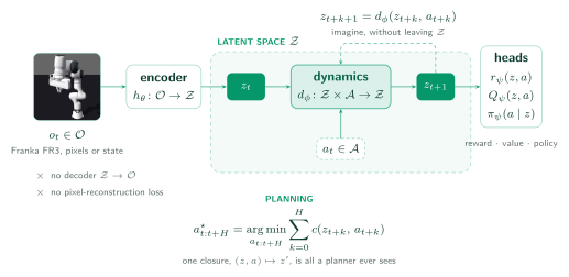
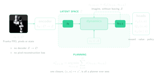
piece	signature	lives in
encoder	\(h: O \rightarrow Z\)	xwm.encoders
dynamics	\(d: Z \times A \rightarrow Z\)	xwm.dynamics
heads	\(Z \rightarrow \mathbb{R}\), \(Z \rightarrow \Delta(A)\)	xwm.heads

There is no decoder \(Z \rightarrow O\) and no pixel-reconstruction loss anywhere in the library. That is a design commitment, not an omission: reconstruction spends capacity on the parts of an observation that are unpredictable and irrelevant (the exact texture of the floor, the grain of a shadow), and a planner never needs them.

Why the dynamics model is the centre

Every family consumes a \((z, a) \rightarrow z\) model, and every planner consumes nothing else:

step = model.dynamics_fn()     # (z, a) -> z'
plan = planner.plan(key, step, model.encode(observation), cost)

Changing family changes how that closure is trained. It never changes how it is used, which is why one implementation of CEM, MPPI, gradient planning and MCTS serves the whole library.

What differs between families

	trains the latent space with	needs reward?	acts by
JEPA	its own future embeddings	no	CEM / MPPI over a latent cost
TD-MPC2	reward + TD value	yes	MPPI over reward + terminal value
MuZero	search-improved targets	yes	MCTS

Read in this order

• 1. Masking

  ---

  What a JEPA is asked to predict, and why the mask has to be hard enough to stop it interpolating from neighbours.

• 2. Collapse

  ---

  Predicting a representation from a representation has a trivial solution. Four ways to forbid it, one of which needs no teacher.

• 3. Planning

  ---

  How a plain closure plus a latent cost becomes a single device call.

• 4. Diagnostics

  ---

  The loss is not the metric. What to measure instead, and what each measure misses.

• 5. Randomness

  ---

  Where key= is optional, where it is mandatory, and why the difference is exactly the jit boundary.