TD-MPC2¶

Latent dynamics trained by reward and temporal-difference value. Where a JEPA learns a representation by predicting its own future embeddings, TD-MPC2 learns one by predicting reward and value. Nothing anchors the latent to the observation except the tasks it has to support, which is the point: the representation keeps exactly what is needed to predict return, and discards the rest.

agent = xwm.families.tdmpc2.tdmpc2(action_dim=7, observation="state", state_dim=20)

Five components over a shared latent¶

component	signature	class
encoder	observation → `z`	`StateEncoder` / `ImageEncoder`
dynamics	`(z, a) → z'`	`MLPDynamics`
reward	`(z, a) → r`	`ScalarHead`
critic	`(z, a) → Q`, pessimistic	`QEnsemble`
policy prior	`z → a`	`GaussianPolicy`

There is no decoder and no reconstruction.

The loss¶

The dynamics unroll horizon steps from a real latent, and three terms are summed per step:

term	compares	default weight
consistency	predicted latent vs the encoded next observation, target detached	`consistency_coef=20.0`
reward	predicted vs observed reward	`reward_coef=0.1`
value	predicted Q vs a TD target from the EMA critic	`value_coef=0.1`

Later steps in the unroll start from a predicted latent, so they are less reliable and count less, so rho=0.5 decays each step's contribution.

The policy is trained separately, to maximise Q with a SAC-style entropy bonus, on detached latents. Its gradient never reshapes the world model, which is what stops a policy from bending the representation toward its own convenience.

loss, metrics = agent.loss(batch, key=key, target=ema_copy)   # the Trainer does this
metrics    # loss_consistency, loss_reward, loss_value, loss_policy, q_mean, entropy, latent_std

Two details do most of the stability work¶

SimNorm latents. SimNorm projects the latent onto a product of simplices, so a long unroll can neither blow up nor collapse. It is a hard constraint, not a penalty.
Categorical reward and value. Both are predicted as distributions over bins (n_bins=101) rather than scalars, using symlog + two-hot targets. That makes the loss scale-free across tasks: a reward of 3 and a reward of 3000 are the same learning problem.

Training it¶

The losses need contiguous slices of a single episode, so this family trains from a ReplayBuffer rather than a shuffled dataset:

buffer = xwm.training.ReplayBuffer(100_000, observation_shape=(20,), action_shape=(7,))

for episode in collect(env):
    # (T + 1) observations for T actions: the last observation is where the
    # last action led. Reward is a first-class field; `extra=` is for anything else.
    buffer.add_episode(episode.observations, episode.actions, episode.rewards)

trainer = xwm.training.Trainer(agent, xwm.training.adamw(3e-4))
state = trainer.init()

for iteration in range(120):
    batch = buffer.sample(batch_size=64, horizon=agent.horizon)
    state, metrics = trainer.step(state, batch, jr.fold_in(key, iteration))

The buffer rejects slices that straddle an episode boundary, since training a dynamics model to predict through a reset is the one transition it can never get right.

uses_target is true for this family, so the Trainer maintains the EMA copy the TD target needs. You do not wire that up yourself.

Acting¶

Two options, and the gap between them is the whole argument for planning:

Plan (MPPI)Policy prior only

planner, cost = xwm.families.tdmpc2.planner(agent, n_samples=512, n_iters=6)
plan = planner.plan(key, agent.dynamics_fn(), agent.encode(observation), cost)
action = plan.actions[0]

action = agent.act(observation)

planner() returns an MPPI already wired to the model's own reward and value heads. Candidates are scored by discounted predicted reward plus a terminal value bootstrap, the term that lets a horizon-3 planner act as though it saw further.

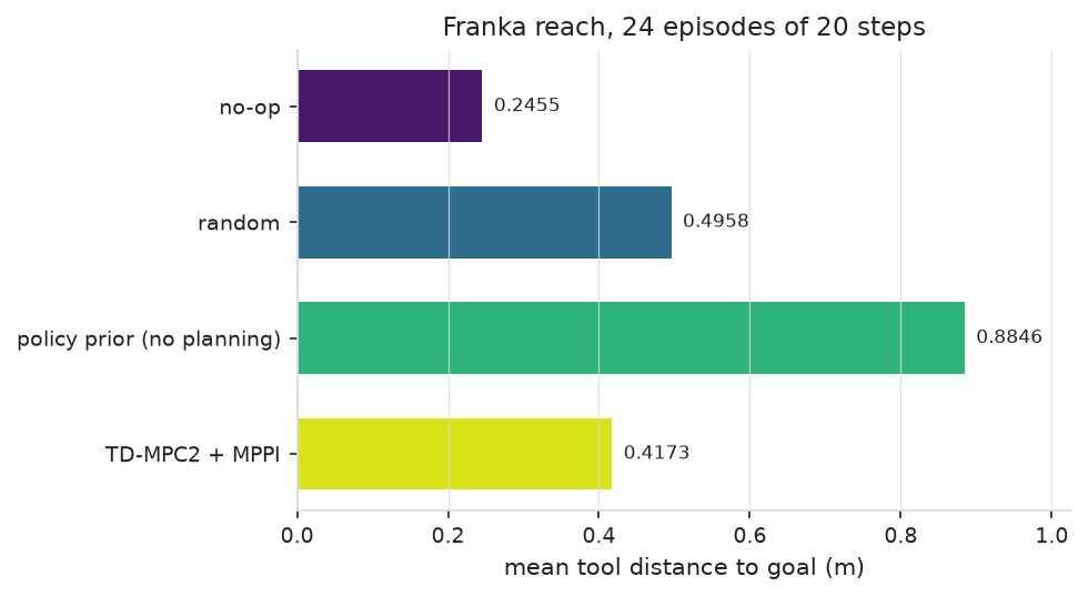
Two runs on the Franka reach task at the identical preset, 120 iterations each (findings):

policy	run A (m)	run A	run B (m)	run B
no-op	0.245	0.0	0.245	0.0
random	0.496	−102.0	0.496	−102.0
policy prior (no planning)	0.894	−264.3	0.885	−260.3
TD-MPC2 + MPPI	0.203	+17.2	0.417	−70.0

The headline result does not reproduce

Identical settings gave +17% in one run and −70% in the other, so the sign of the effect is not determined by the configuration. Do not quote either number as the result. In run B the consistency loss rose throughout training, from 0.87 to 1.68, so the planner was working through latent dynamics that were degrading under the very term meant to sharpen them.

What survives both runs is the planner-against-prior gap: planning is 2.1 to 4.4 times closer to the goal than the policy prior alone, and the prior is worse than random actions either way. The prior is a proposal distribution, not a controller, which is exactly the role TD-MPC2 assigns it. Whether the planner on top of it beats doing nothing is, at this budget, a coin flip.

TD-MPC2 policy comparison — Run B. Distances are ground truth; the agent only ever sees reward.

Eight frames of a TD-MPC2 planning episode — One planning episode, sampled evenly across its 21 steps rather than at the start, so it shows the whole motion. Rendered at 768 px per frame, so open it full size to see the arm extend.

Starting from a JEPA¶

agent = xwm.families.tdmpc2.tdmpc2(action_dim=7, encoder=pretrained_jepa.encoder)

The encoder is trainable by default here, because the consistency term needs to be able to move the latent, but starting from a representation that already separates observations is strictly easier than starting from noise.

Example¶

examples/07_tdmpc2_franka.py runs the loop above on the Franka arm: collect, train, plan, and compare against no-op, random and the policy prior. See Examples.