Generalized simulated annealing

Tsallis & Stariolo's algorithm is two qjax calls, and its cooling schedule is a ratio of two q_log calls whose \(q\to1\) limit is exact. What the benchmark then measures is a negative result with a mechanism — and it is reported as one.

What it shows

Generalized simulated annealing (Tsallis & Stariolo, Physica A 233, 395, 1996 — this journal's own lineage) replaces the two Boltzmann ingredients of classical annealing by their \(q\)-deformed counterparts:

ingredient	classical	generalized	in qjax
proposal	Gaussian	\(q\)-Gaussian, tails $\sim	x
acceptance	\(e^{-\Delta E/T_A}\)	\(\exp_{q_A}(-\Delta E/T_A)\)	qjax.q_exp(-delta / t_a, q_a)
schedule	Geman–Geman \(\ln\)	the Tsallis law below	qjax.physics.visiting_temperature

Setting \(q_V = q_A = 1\) recovers Kirkpatrick's Boltzmann machine exactly, and \(q_V = 2\) is Szu & Hartley's Cauchy machine, so the \(q = 1\) arm is a genuine baseline rather than a strawman.

The schedule is where the library earns its place

The Tsallis cooling law

\[T_q(t) = T_q(1)\,\frac{2^{q-1}-1}{(1+t)^{q-1}-1}\]

is \(0/0\) at \(q = 1\) — the same pathology qjax.shared.series exists to defeat. Substituting \(x^{q-1} - 1 = (q-1)\ln_{2-q}x\) cancels both \((q-1)\) factors and leaves a ratio of two q_log calls:

def tsallis_schedule(step, initial, q):
    return initial * qjax.q_log(2.0, 2.0 - q) / qjax.q_log(1.0 + step, 2.0 - q)

At \(q = 1\) this returns the Geman–Geman logarithmic schedule \(T(1)\ln 2/\ln(1+t)\) to zero error, with no branch on \(q\) and — because q_log carries the limit through the entire function \((e^t-1)/t\) rather than switching to a \(q\)-independent formula — with a correct, non-zero derivative in \(q\). The test suite pins the limit to \(10^{-12}\) and checks \(\partial T/\partial q\) at \(q=1\) against its analytic value \((\ln 2/\ln(1+t))(\ln 2 - \ln(1+t))/2\). A learnable cooling index is therefore just another parameter.

How it works

import qjax.physics as qp

visiting = qp.visiting_temperature(step, INITIAL_VISITING, q_visit)
accepting = qp.acceptance_temperature(step, INITIAL_ACCEPTANCE, q_accept)

# Tsallis & Stariolo tie the width to T_V^{1/(3-q_V)}, not to T_V.
width = visiting ** (1.0 / (3.0 - q_visit))
jump = direction * jnp.abs(qjax.sample(key, q=q_visit, beta=1.0 / width**2, shape=()))

probability = jnp.minimum(qjax.q_exp(-(new - old) / accepting, q_accept), 1.0)

Two implementation details are measured rather than assumed:

• The proposal must be isotropic — one unit direction in the full \(3n\)- dimensional configuration space times one radial draw. Drawing the \(3n\) coordinates independently looks equivalent and is not: at \(q_V = 2.7\) each coordinate exceeds 100 width units with probability \(\approx 0.09\), so across 39 coordinates something blows up on essentially every step, and LJ13 loses more than half its depth.
• The walk is confined to a ball, and the proposal is capped at its diameter. That cap is exact (a longer displacement is projected to the same place) and it is necessary: qjax.sample builds the Student-\(t\) from a \(\chi^2_\nu\) variate, and in float32 a shape-0.09 gamma draw underflows to exactly zero often enough (about 1 in 2000 at \(q_V = 2.7\)) that the division returns +inf.

Result

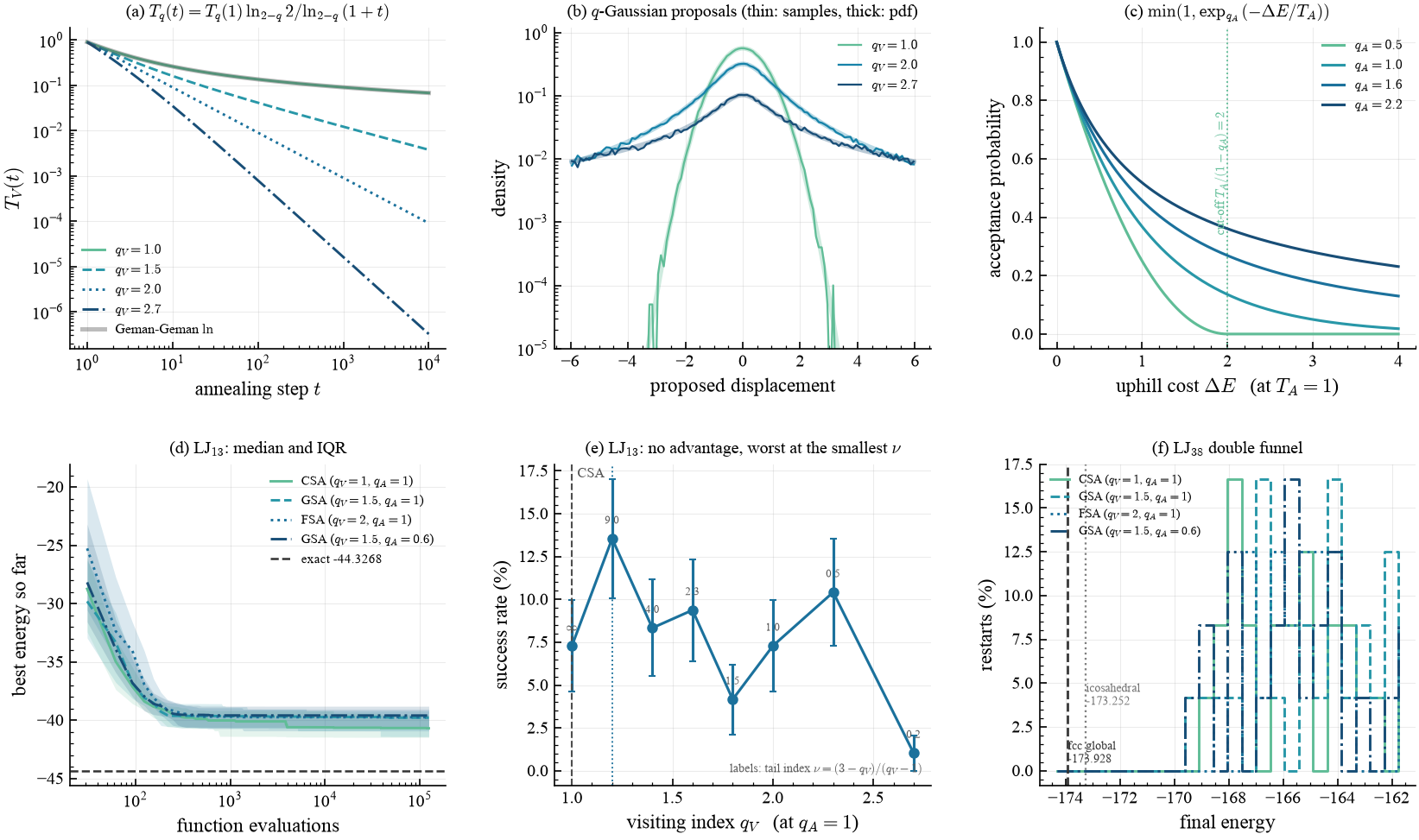
(a) The Tsallis schedule for several \(q_V\), with the Geman–Geman logarithmic curve underneath the \(q_V=1\) case — they coincide exactly. (b) \(q\)-Gaussian proposals: sampled histograms (thin) on the analytic density (thick), validating qjax.sample and showing the Lévy-like tails. (c) The acceptance rule, with the \(q_A<1\) cut-off at \(\Delta E = T_A/(1-q_A)\) marked — that cut-off is physics, not underflow. (d) LJ13 best-so-far energy against function evaluations, median and interquartile range. (e) The visiting-index scan, labelled with the tail index \(\nu\). (f) LJ38: where each arm ends up, relative to both funnel minima.

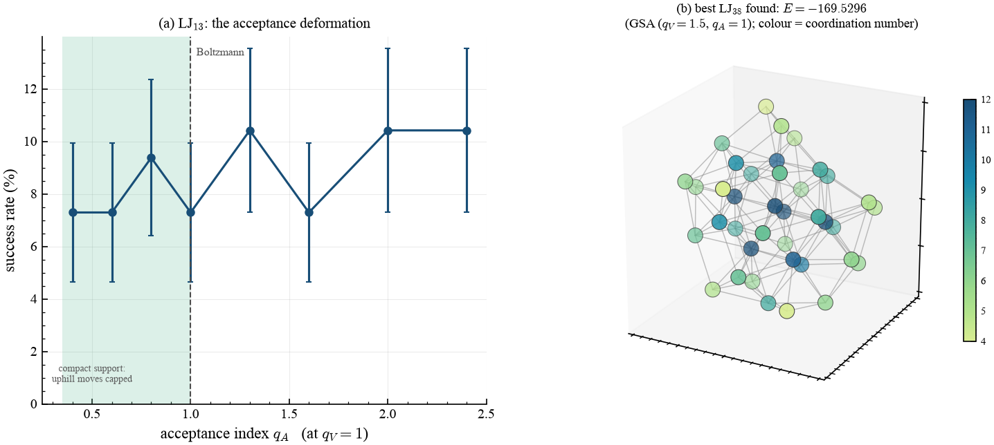
(a) The companion scan over the acceptance index at \(q_V = 1\), isolating the second deformation. The shaded region is the compact-support side, where an uphill move beyond \(T_A/(1-q_A)\) is rejected outright. (b) The best LJ38 cluster found, bonded within \(1.35\,\sigma\) and coloured by coordination number.

Both scans are 1-D on purpose. A \((q_V, q_A)\) grid is the tempting figure and the wrong one: at any trial count this script can afford, a single cell carries a binomial error of order 12 percentage points — larger than any effect being looked for — so it renders as a blocky pattern that invites over-reading. Scanning each index separately at six times the restarts gives error bars small enough to mean something.

Validation

quantity	measured	reference	source
LJ2 (regular simplex at \(2^{1/6}\sigma\))	−1.000000000	−1	closed form
LJ3	−3.000000000	−3	closed form
LJ4	−6.000000000	−6	closed form
LJ7 best found	−16.505390	−16.505384	Cambridge Cluster Database
LJ13 best found	−44.326805	−44.326801	"
LJ38 best found	≈ −169.5	−173.928427	" (budget insufficient — see below)
\(T_q(t)\) at \(q=1\) vs Geman–Geman	0 error	—	closed form
\(\partial T_q/\partial q\) at \(q=1\)	matches to \(10^{-6}\)	—	closed form

The three closed forms are exact to \(10^{-12}\), and both LJ7 and LJ13 global minima are recovered to better than \(10^{-4}\) — including the sign check that matters: no arm ever reports an energy below its tabulated reference, which a buggy potential or an active confining wall would produce immediately.

The measured result

Success rates within \(10^{-2}\) of the reference, laptop tier:

system	CSA (\(q_V=1\))	GSA (\(q_V=1.5\))	FSA (\(q_V=2\))	GSA (\(q_V=1.5\), \(q_A=0.6\))
LJ7 (32 restarts)	31.2 ± 8.2 %	28.1 ± 7.9 %	34.4 ± 8.4 %	21.9 ± 7.3 %
LJ13 (64 restarts)	17.2 ± 4.7 %	12.5 ± 4.1 %	4.7 ± 2.6 %	9.4 ± 3.6 %

Deforming the visiting distribution does not accelerate global optimization here. On LJ13 the classical Gaussian proposal has the highest success rate of the four arms and the Cauchy machine is the lowest, \(2.3\sigma\) apart; LJ7 is flat within its error bars.

The two scans, at 96 restarts each, say the same thing more sharply. They use a smaller per-restart budget than the four arms above (2500 steps against 4000), so their absolute rates are lower and the two sets should not be compared directly — only within themselves.

scan	at the classical point	best in the scan	worst in the scan
visiting \(q_V\) (at \(q_A=1\))	7.3 ± 2.7 %	13.5 ± 3.5 % at \(q_V=1.2\) (\(\nu=9\))	1.0 ± 1.0 % at \(q_V=2.7\) (\(\nu=0.18\))
acceptance \(q_A\) (at \(q_V=1\))	7.3 ± 2.7 %	8.0 % mean over \(q_A<1\)	9.6 % mean over \(q_A>1\)

Read together: the visiting index is flat within error for \(q_V \lesssim 2\), and \(q_V = 2.7\) is worse than every other point by more than \(2\sigma\). The acceptance index does essentially nothing — the compact-support and heavy-tailed sides differ from Boltzmann by less than one standard error. So of the two deformations that generalized annealing introduces, one is inert here and the other only hurts, once its tail index gets small enough. There is no interior optimum to report.

The reason is not the width — the Tsallis–Stariolo coupling \(\sigma = T_V^{1/(3-q_V)}\) is used, and its exponent already shrinks the width faster at large \(q_V\) — but the tail index

\[\nu = \frac{3-q_V}{q_V-1},\]

which sets how often a proposal is catastrophic: a displacement exceeds \(k\) width units with probability \(\sim k^{-\nu}\). At \(q_V = 2.7\), \(\nu = 0.18\), and a majority of proposals then exceed the container diameter however small the width is (measured, and asserted in the test suite), so the cluster is scattered at every step and the cooling schedule never gets to act.

What this is and is not

This is a statement about this parameterization, not a refutation of Tsallis & Stariolo. Three things differ from their setup, and any of them could matter: the proposal is an isotropic radial \(q\)-Gaussian rather than their exact \(D\)-dimensional visiting distribution, the local minimizer is Adam rather than a quasi-Newton method, and the cluster is confined to a ball. What the example does establish is that the entropic index is not a free win on this landscape, and that \(\nu\) — not \(q_V\) — is the quantity to reason about when choosing it.

LJ38 is not solved, deliberately

LJ38's global minimum is an fcc truncated octahedron, not icosahedral, and the much wider icosahedral basin at \(-173.252378\) is only 0.38 % higher in energy. Nothing in a budget of \(10^4\)–\(10^5\) evaluations reliably finds it; at the laptop tier no arm even reaches the icosahedral funnel. The panel is therefore framed as a funnel-escape distribution against both minima, and the rates are reported as measured. Promising otherwise would be the easiest place in this whole set of examples to mislead.

Takeaways

• GSA is two qjax calls; its schedule's \(q\to1\) limit is exact and differentiable through q_log, with no branch.
• The LJ potential and the two smaller global minima validate to machine precision, so the negative result rests on a verified implementation.
• The visiting index is not a free win: on LJ clusters the classical proposal is at least as good, and performance degrades as the tail index \(\nu\) falls.
• Reason about \(\nu\), not \(q_V\): it is the parameter with operational meaning, and it changes by a factor of 50 across \(q_V \in [1.2, 2.7]\).

References

• C. Tsallis & D. A. Stariolo, Generalized simulated annealing, Physica A 233, 395 (1996).
• H. Szu & R. Hartley, Fast simulated annealing, Phys. Lett. A 122, 157 (1987).
• S. Geman & D. Geman, IEEE Trans. Pattern Anal. Mach. Intell. 6, 721 (1984).
• D. J. Wales & J. P. K. Doye, Global optimization by basin-hopping, J. Phys. Chem. A 101, 5111 (1997); and the Cambridge Cluster Database.
• J. P. K. Doye, M. A. Miller & D. J. Wales, The double-funnel energy landscape of the 38-atom Lennard-Jones cluster, J. Chem. Phys. 110, 6896 (1999).