Anomalous diffusion

Here \(q\) is neither chosen nor learned — it is measured, from trajectories, with a value predicted in advance and two independent estimators that can disagree.

What it shows

Nonextensive statistics makes a falsifiable prediction about anomalous diffusion. The nonlinear (porous-medium) Fokker–Planck equation

\[\frac{\partial p}{\partial t} = D\,\frac{\partial^2 p^{\,2-q}}{\partial x^2}\]

has the self-similar \(q\)-Gaussian solution of Tsallis & Bukman (1996), whose width obeys \(\langle x^2\rangle \propto t^{\alpha}\) with

\[\alpha = \frac{2}{3-q}.\]

So the shape of the distribution and the growth of its width are not two free parameters: either one predicts the other. Fitting \(q\) to the density and reading it off the mean-squared displacement are therefore independent measurements of the same number.

A second, experimentally realized mechanism gives the same distribution from a linear-noise Langevin equation with saturating (Sisyphus) friction,

\[dp = -\frac{\alpha\,p}{1 + (p/p_c)^2}\,dt + \sqrt{2D_0}\,dW,\]

whose exact stationary solution is a \(q\)-Gaussian with

\[q = 1 + \frac{2D_0}{\alpha\,p_c^2}, \qquad \beta = \frac{\alpha}{2D_0}.\]

The heavy tail comes entirely from the friction saturating, so a fast atom is barely damped — the noise stays ordinary and Gaussian. Because the three coefficients are ours to choose, the true \(q\) is known to machine precision. Separately, Lutz (2003) evaluated those coefficients semiclassically for atoms in a dissipative optical lattice and obtained \(q = 1 + 44\,E_R/U_0\), confirmed experimentally by Douglas, Bergamini & Renzoni (2006). The two are kept distinct: the first is exact for our simulation, the second is a prediction about a real experiment.

How it works

The fit is the idiom of fitting \(q\) by maximum likelihood, with an error bar added, because the comparison against theory has to be quantitative:

import qjax
from qjax.nn import bounded_q

def negative_log_likelihood(raw):
    q, beta = bounded_q(raw[0], 1.0, 2.9), jax.nn.softplus(raw[1]) + 1e-3
    return -jnp.mean(qjax.q_gaussian_logpdf(samples, q, beta))

# ... gradient descent, then the asymptotic Fisher covariance at the optimum:
covariance = jnp.linalg.inv(jax.hessian(negative_log_likelihood)(raw)) / n
sensitivity = jax.jacfwd(lambda r: bounded_q(r[0], 1.0, 2.9))(raw)
q_sigma = jnp.sqrt(sensitivity @ covariance @ sensitivity)

qjax.sample also supplies the initial condition for its own equation: starting the superdiffusive run on the exact self-similar \(q\)-Gaussian profile makes the mean-squared displacement a pure power law from the first step, which moves the fitted exponent from 1.246 to 1.324 against the exact \(4/3\).

Two constraints, stated rather than hidden

• For \(q < 1\) the \(q\)-Gaussian has compact support, so q_gaussian_logpdf is \(-\infty\) outside it and the likelihood is \(+\infty\): a gradient-based fit started at \(q > 1\) can never cross into \(q < 1\). The subdiffusive arm's index is therefore measured through \(q = 3 - 2/\alpha\) instead. That is a real property of compact-support likelihoods.
• bounded_q maps onto an open interval, so \(q = 1\) is approached and never attained. For genuinely Boltzmann–Gibbs data the fit lands a little above the boundary (\(\approx 1.04\) at the default step count), so the control's \(\hat q\) reads as an upper bound, not an unbiased estimate.

Result

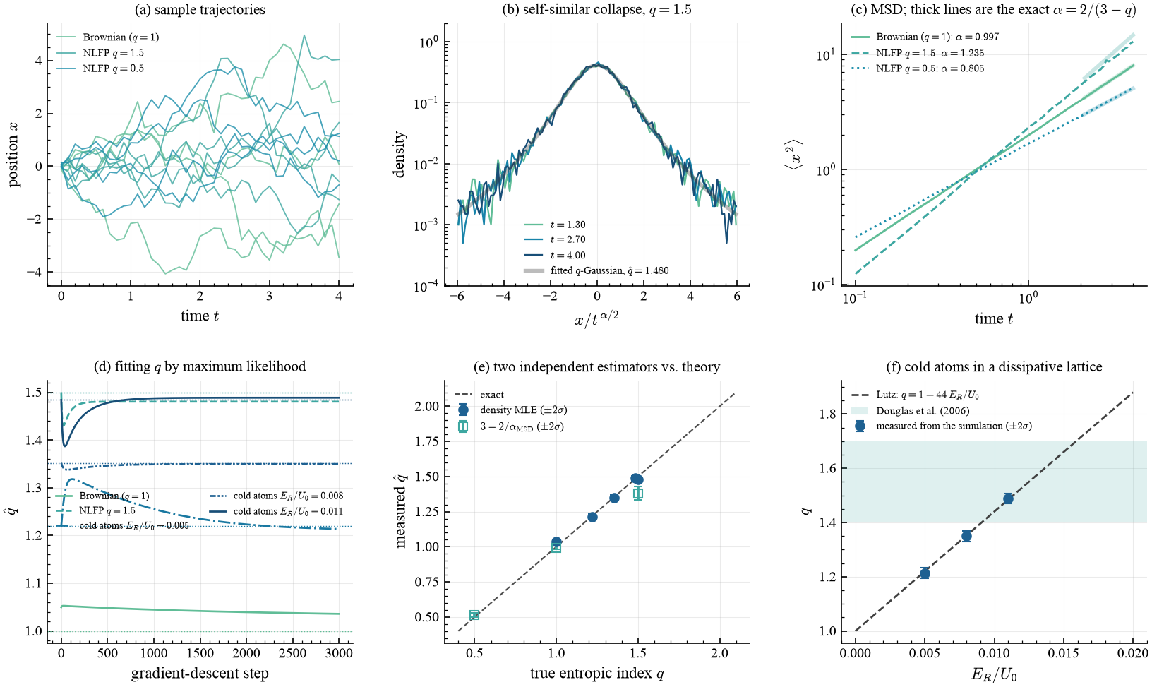
(a) Sample trajectories: sub-, normal and superdiffusive are visibly different. (b) The self-similar collapse — densities at three times, rescaled by \(t^{\alpha/2}\), falling onto one curve, with the arm's own fitted \(q\)-Gaussian transported into the rescaled coordinate. (c) Mean-squared displacement with the exact \(\alpha = 2/(3-q)\) reference slopes overlaid. (d) The maximum-likelihood run for each arm, with theory dashed. (e) The money panel: two independent estimators against the known \(q\), on the identity line. (f) The cold-atom arms against Lutz's law and the range reported by Douglas et al.

Validation

Laptop tier (20 000 particles), against exact values:

arm	true \(q\)	\(\hat q\) from the density	\(\hat q\) from the MSD	\(\alpha\) measured / exact
Brownian control	1.0000	1.036 ± 0.009 (upper bound)	0.994 ± 0.006	0.9971 / 1.0000
NLFP \(q=1.5\)	1.5000	1.4804 ± 0.0090	1.381 ± 0.024	1.235 / 1.3333
NLFP \(q=0.5\)	0.5000	n/a (compact support)	0.5142 ± 0.0074	0.8046 / 0.8000
cold atoms, \(E_R/U_0 = 0.005\)	1.2200	1.2138 ± 0.0103	n/a (stationary)	n/a
cold atoms, \(E_R/U_0 = 0.008\)	1.3520	1.3499 ± 0.0097	n/a (stationary)	n/a
cold atoms, \(E_R/U_0 = 0.011\)	1.4840	1.4886 ± 0.0090	n/a (stationary)	n/a

All three cold-atom indices land within one sigma of the exact stationary value, which is simultaneously Lutz's prediction for that lattice depth. The Brownian control returns \(\alpha = 1.00\) to \(0.3\,\%\), and the subdiffusive arm's scaling-relation estimate is within \(2\sigma\) of the exact \(q = 0.5\).

Having two independent estimators means they can disagree, and on the superdiffusive arm they do: the density likelihood gives \(1.480 \pm 0.009\) (\(2.2\sigma\) from \(1.5\)) while the mean-squared-displacement exponent gives \(\alpha = 1.235\) against the exact \(4/3\) — about \(7\,\%\) low. The distribution reaches its self-similar shape long before the width reaches its asymptotic slope, so within the simulated window the MSD route is the slower of the two to converge. Reporting both is the point; a single fitted exponent would have looked like agreement.

The mean-squared-displacement route is deliberately marked n/a for the cold-atom arms: they relax to a stationary momentum distribution, so the second moment saturates instead of growing and \(\alpha = 2/(3-q)\) does not apply. That is also true of the real experiment, where the velocity distribution is the observable.

Equilibration is the hard part

The cold-atom arms are run for a matched number of friction relaxation times rather than a matched number of steps, because the friction differs fourfold across them. It matters, and the reason is physical: past \(q = 5/3\) the \(q\)-Gaussian's second moment diverges and the tail of the stationary state equilibrates as a power law rather than exponentially. At \(q = 1.75\) the measured index is still 3 % low after 150 relaxation times and creeping upward; the arms here stay below \(5/3\) so that the error bars mean what they say.

Takeaways

• \(q\) can be a measured physical quantity with an error bar, not a hyperparameter.
• Two independent estimators — the density likelihood and the MSD exponent — agree with an exactly known \(q\), and the relation \(\alpha = 2/(3-q)\) ties them.
• Heavy tails need not come from heavy-tailed noise: saturating friction with ordinary Gaussian noise produces an exact \(q\)-Gaussian.
• The compact support of the \(q<1\) \(q\)-Gaussian is a real obstacle to likelihood-based inference, and the scaling relation is the way around it. It is not an obstacle to a PDE residual, which is well defined there — see the PINN, which solves this same equation from the other side — and where a second, unrelated entropic index turns up in the distribution of those residuals.

References

• A. R. Plastino & A. Plastino, Non-extensive statistical mechanics and generalized Fokker-Planck equation, Physica A 222, 347 (1995).
• C. Tsallis & D. J. Bukman, Anomalous diffusion in the presence of external forces, Phys. Rev. E 54, R2197 (1996).
• E. Lutz, Anomalous diffusion and Tsallis statistics in an optical lattice, Phys. Rev. A 67, 051402(R) (2003).
• P. Douglas, S. Bergamini & F. Renzoni, Tunable Tsallis distributions in dissipative optical lattices, Phys. Rev. Lett. 96, 110601 (2006).